Political Stances: Support Vector Machines
Overview
The Support Vector Machine (SVM) preforms linear classification (among with other kernels) to project the data into classifications, based on their long vector inputs. Applying this model to text data may allow for classification of unlabeled text. This classification is based in Vapnik’s statistical learning theory which has provided insight into the classification of text. These methods inform the ability to understand nuance and future action of a particular text. For exampale, the query ‘using support vector machines to predict the future’ generates over one million citations on Google Scholar. Specifically in the context of bills, it may be insightful to understand the characteristics and similarities to understand how bills change and evolve both spatially and temporally. Applying SVM to news data may provide insights into media bias as well. How are certain features in the news cycle represented differently by different sources and within different contexts? Applyinng SVM in for this case will provide insight into differences of language when reporting on partisian issues and how this polarization (may or may not) be present in proposed climate oriented bills.
Table of Contents
- Sentiment Analysis
- Data Preparation
- Method
- Model Evaluation
- Assessing the Preformance of SVM Models
- Assessing the Classifications of the Polynomial Cost 1000 SVM
- Conclusions
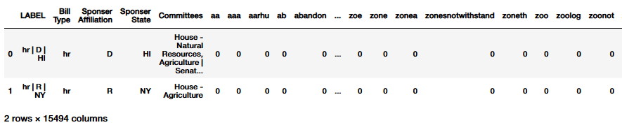
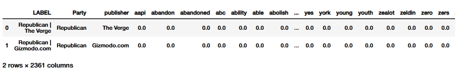
The data utilized in this method is similar to that of the other machine learning methods applied. A lemmatized version of the Count Vectorizer was utilized. This data may be found at my Hugging Face Collection.
Illustrated below is the dataframe which stores the counts utilized to calculate probabilities which help the model ‘learn’. Described in the following sections is the steps used to generate a sentiment label for each of the text files and then the additional data preparation for supervised learning.
Sentiment Analaysis
The sentiment was calculated for all news articles and climate bills in an attempt to generate a classifier which preforms well on sentiment. This decision was motivated as it may be interesting to train a classifier - in addition to the tools already provided - in an attempt to identify nuance within sentiment. To generate a sentiment label to compliment the eight labels in the data already, NLTK was utilized. The Seniment Intensity Analyzer from the Vader attribute was utilized to generate a numerical score referred to as the ‘compound’. It illustrates how strong a particular emotion is throughout the text.
The analyzer was instantiated through a non-paramaratized call and then wrapped into a function:
from nltk.sentiment import SentimentIntensityAnalyzer
sia = SentimentIntensityAnalyzer()

def word_scorer(x):
    sentiment = sia.polarity_scores(text=x)
    return (sentiment['compound'])

def sentiment_translator(x):
    if x >= 0.7:
        return ("Positive")

    else:
        return ("Negative")
 This is a portion of the combined text that was generated from the CountVectorizer counts. This function utilized *x* as an input, which would then be lambda applied to an alphabatized text string (as the data was reconstructed from the Count Vectorizer counts). This generated a sentiment value column, which would then be converted using the *sentiment_translator* into a categorical label. The threshold of 0.7 was selected after an exploratory analysis of both the data and the distribution of sentiment.
Sentiment Distribution for the Testing Dataset
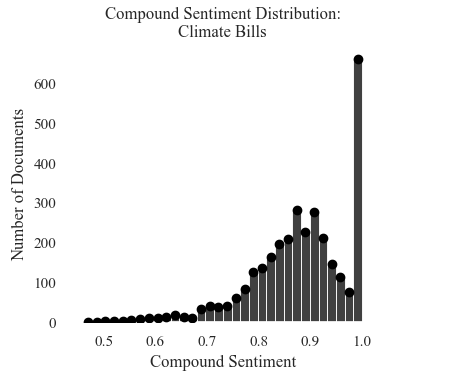
Sentiment Score Distribution: Proposed Climate Bills
The distribution matches the news headlines, but has an overwhelming about of positive samples. There is a long skewed tail beginning at 0.7 valence.
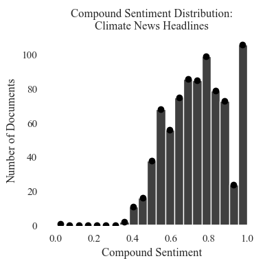
Sentiment Score Distribution: News Headlines
The scores are a negatively skewed (right leaning not sentiment negative!) modal distribution. The majority of the sample have an strong positive average.
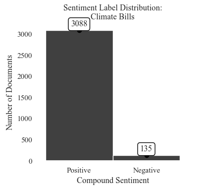
Sentiment Label Distribution: Proposed Climate Bills
The distribution is uneven with 135 negative instances and 3,088 positive instances. This may cause later classification issues.
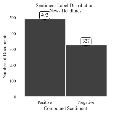
Sentiment Label Distribution: News Headlines
The distribution is mor equal than the climate bills with 492 positive instances and 327 negative instances
Data Preparation
| Training Data | Testing Data | |
|---|---|---|
| News Headline: Partisian Affiliation | 573 | 246 |
| News Headlines: Publisher | 573 | 246 |
| News Headlines: Publisher and Partisian Affiliation | 573 | 246 |
| News Headlines: Sentiment | 573 | 246 |
| Climate Bills: Sponsor Affiliation | 2256 | 967 |
| Climate Bills: Sponsor State | 2256 | 967 |
| Climate Bills: Metadata | 2256 | 967 |
| Climate Bills: Bill Type | 2256 | 967 |
| Climate Bills: Hearing Committee | 2256 | 967 |
| Climate Bills: Sentiment | 2256 | 967 |
Method
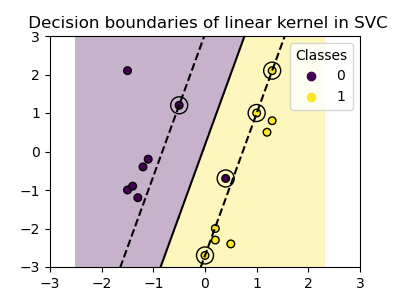
Linear Kernel
Polynomial Kernel
Radial Basis Function Kernel
Image Source: Plot Classification Boundaries with Different SVM Kernels
Multiple Kernels and costs were tested to exhaust the possibilities of the model. The linear kernel was selected because of its simplicity. It draws a line through the data in order to separate the paritions. Next, the polynomial kernel was selected in an attempt to provide the model with forgiveness in real-life language, as often polarization and text labels are more nuanced than the binary. The third kernel selected was Radial Basis Kernel (RBF), which generates data clusters. This kernel was selected to continue the clustering methods applied earlier in the project, and to also identify more nuance between multi-dimensional labels.
svm_model = sklearn.svm.SVC(C=100, kernel = 'rbf', degree = 3, gamma = 'scale', verbose = True)
The SVM model instantiation, through SciKitLearns Support Vector Classification function. The cost was changed iteratively to either 100 or 1000. The intution behind cost is its use for regularizaiton. This is then multiplied by the loss function and penalty in order to classify the instance. High cost was set in this model in order to control for the high dimensionality present in the data. The gamma was set to scale in an attempt to control for the kernel coefficient systematically across the data. This is also the rational for keeping the degree set at 1, which represents fair linearity across the different models. The findings below are a comparison of cost - not how other parameters are changed.
Similar to Naïve Bayes and Decision trees, an SVM modeler function was generated. The change in this function is that it requires an SVM model. This was used in order to easily change the parameters needed for the model.
def svm_modeler(svm_model, data_train, labels_train, data_test, labels_test, label_column_name,
                graph_title, labels_name, file_name,filter_top_n = False, N=10 ,fig_x = 6, fig_y = 4):
    data_train = data_train.drop(columns = label_column_name).copy()
    data_test = data_test.drop(columns = label_column_name).copy()

    feature_names_train = list(data_train.columns)
    feature_names_test = list(data_test.columns)

    ## These may be edited depending on the test

    ## Fitting the data
    svm_model.fit(data_train, labels_train)

    ## Creating predictions
    predictions = svm_model.predict(data_test)


    ## Assessing the models abilitiy
    accuracy, precision, recall = model_verification(labels_test, predictions)

    ## Filtering for Clean Visualizations
        ## Filtering for Clean Visualizations
    if filter_top_n:
        # Call filter_top_n_labels to get filtered labels and predictions
        labels_test_filtered, predictions_filtered = filter_top_n_labels(labels_test, predictions, N)

        # If data remains after filtering, create the filtered confusion matrix
        if len(labels_test_filtered) > 0 and len(predictions_filtered) > 0:
            visual_confusion_matrix(labels_test_filtered, predictions_filtered,
                                    f"{graph_title} (Top {N})", labels_name,
                                    f"filtered_{file_name}", fig_x, fig_y)
        else:
            print(f"[Warning] No data left after filtering top {N} labels — skipping confusion matrix.")
    else:
        # If no filtering is needed, generate confusion matrix with all data
        visual_confusion_matrix(labels_test, predictions, graph_title, labels_name, file_name, fig_x, fig_y)

    return (accuracy, precision, recall)
The same evaluation metrics (accuracy, recall, and precision) were generated using the functions described in Naive Bayes. The definition of these metrics are provided at length in its own section on the page. The confusion matricies where generated in the same way in order to compare between the models in the final conclusions.
Assessing the Preformance of Multiple Iterations of SVM
Across all tests, the relative performance of different labels is similar. The Sentiment classification has the highest accuracy with a range between 93% and 94% for Climate Bills. The precision and recall mirror these patterns with the same rate of prediction. The News headlines have a larger range between 89% and 90%. Precison tends to be above the accuracy, ranging between 82% - 94%. The recall is much lower, yet comparable to the scores of the other ‘well’ preforming labels in the news data. It ranges from 58% to 66%. The model had similar preformance trends to that of the Naive Bayes model and the same labels.
Linear Kernel with Cost 100
The average accuracy between the Linear Models is the same at 56%. The average precision is 43.4% and the average recall is 43.2%.

Linear Kernel with Cost 1000
There is no observed difference between the varying costs in any evaluation metric.
Polynomial Kernel with Cost 100
The average accuracy is 54.5%, average precision is 45.9%, and average recall is 40.8%.
Polynomial Kernel with Cost 1000
The average accuracy is 56.1%, average precision is 46.1%, and average recall is 42.7%.
RBF Kernel with Cost 100
The average accuracy is 49.4%, average precision is 48.2%, and average recall is 40.8%.
RBF Kernel with Cost 1000
The average accuracy is 49.5%, average precision is 43.2%, and average recall is 42.6%.
So… what is the best model? The polynomial kernel with cost 1000. The data was paritioned using a “U” like concave into the other classification. This works particulary well for this type of data because in some cases, the labels are binary - in addition, the few testing instances that are negative may make their features more salient because they are more unique in this way. To keep the discussion concisce, only the results from this particular model will be reported. If desired, the outputs from the models are all listed in the GitHub version of the code notebook.
Assessing the Classifications of the Polynomial Cost 1000 SVM
The patterns illustrated here are generated from the Polynomial Cost 1000 SVM. In this case, the patterns are illustrated only in some of the labels because of the length and commplexity of the confuson matrix. In addition the accuracy of the publisher and affiliation, bill metadata, and bill committee scored low on preformance. This suggests that even if there were patterns identified, they may not have actually been learning, and the classifier managed to get a few lucky guesses.
The patterns illustrated in the confusion matricies show minimal learning for the publisher of the news data and the bill sponsor states. The strongest learning is illustrated through sentiment. This may be in part due to the distribution of the training data, and the relatively positive valence scores generally.
News: Publisher
The model did not learn properly, and predicted the majority of the labels to be of FreeRepublic.Com. This was illustrated similarly in the Naive Bayes modeling.
News: Partisian Affiliation
The model tended to predict more labels 'Democrat', and predict more 'Democrat' labels than Republican labels.
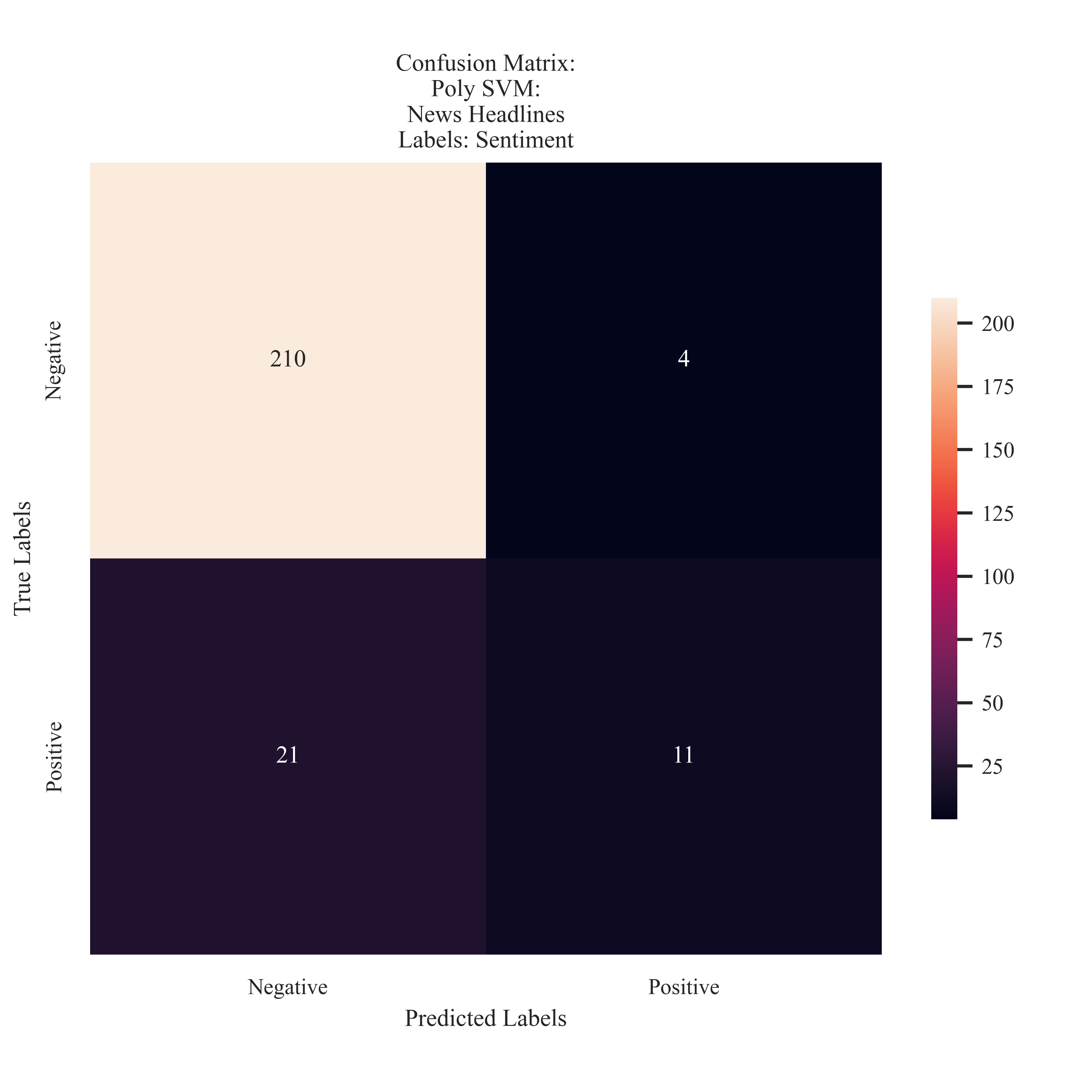
News: Sentiment
The model preferred to predict negative sentiment, however through counts, it is clear that the majority of the testing set was negative labels.
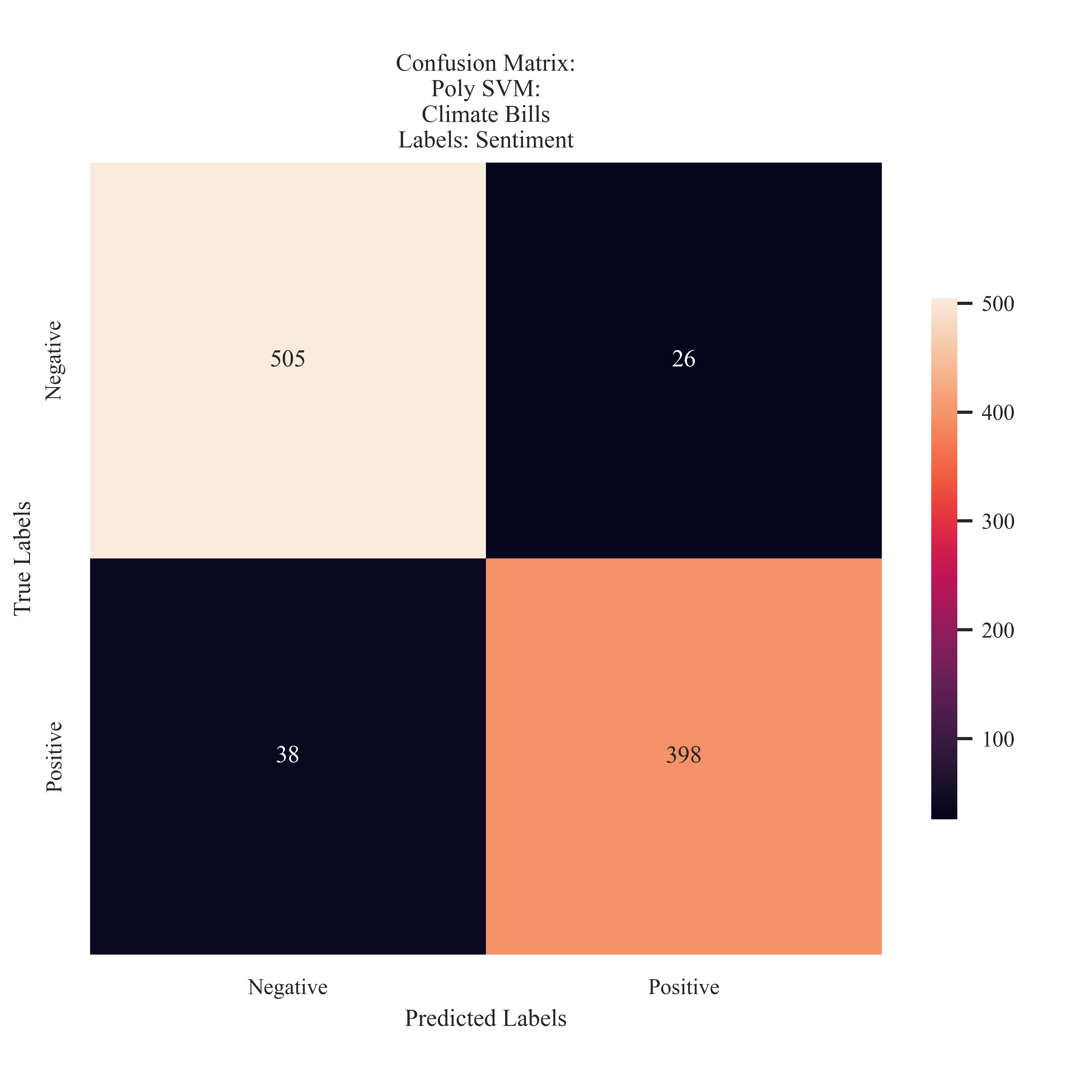
Climate Bills: Sentiment
The classifier preformed accurately when predicting sentiment and only misclassified 6% of the testing instances.
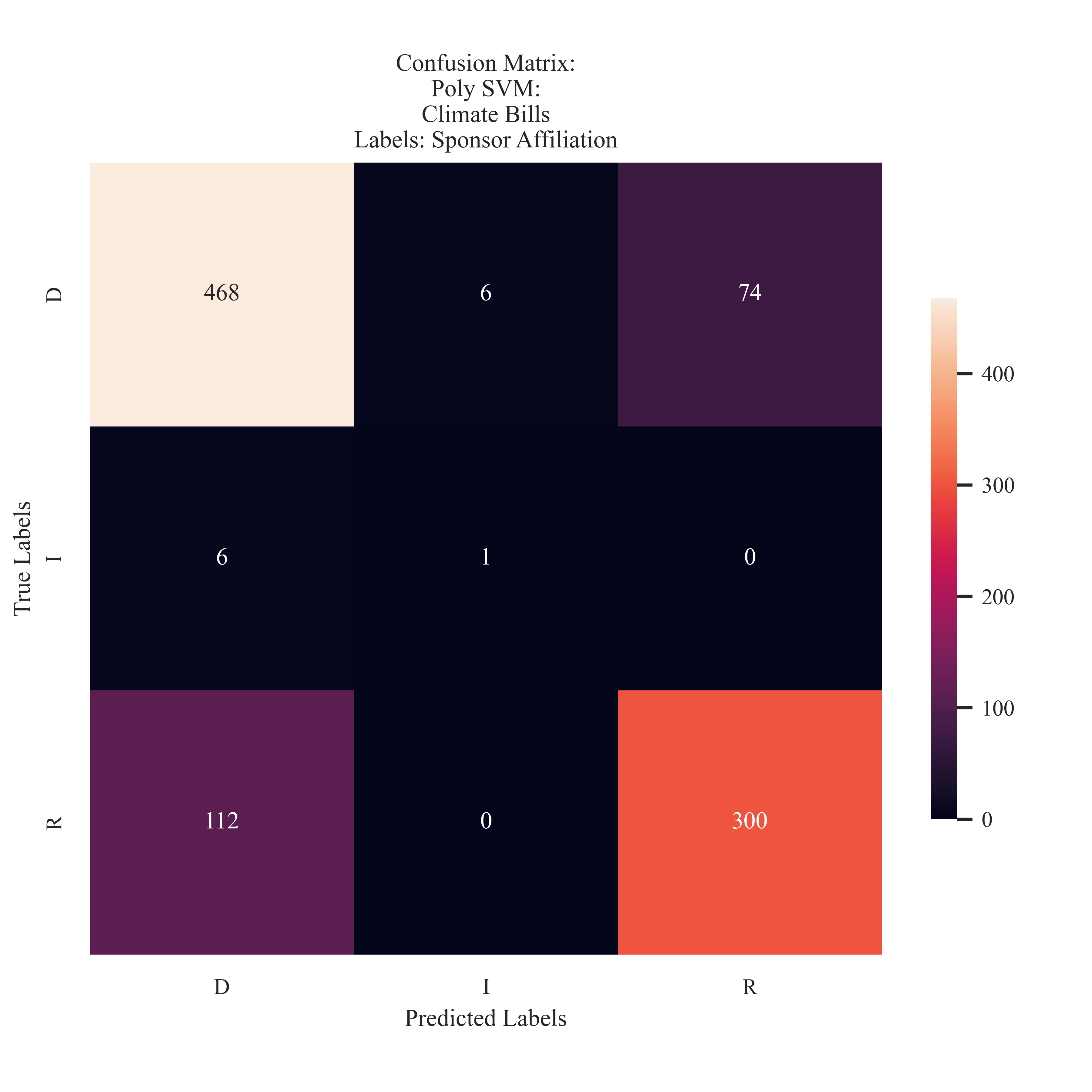
Climate Bills: Sponsor Affiliation
The model strugged with predicting the Independent proposed bills, however, preformed better in comparison to the Naive Bayes model. The SVM model preferred to predict Democrat labels over Republican labels.
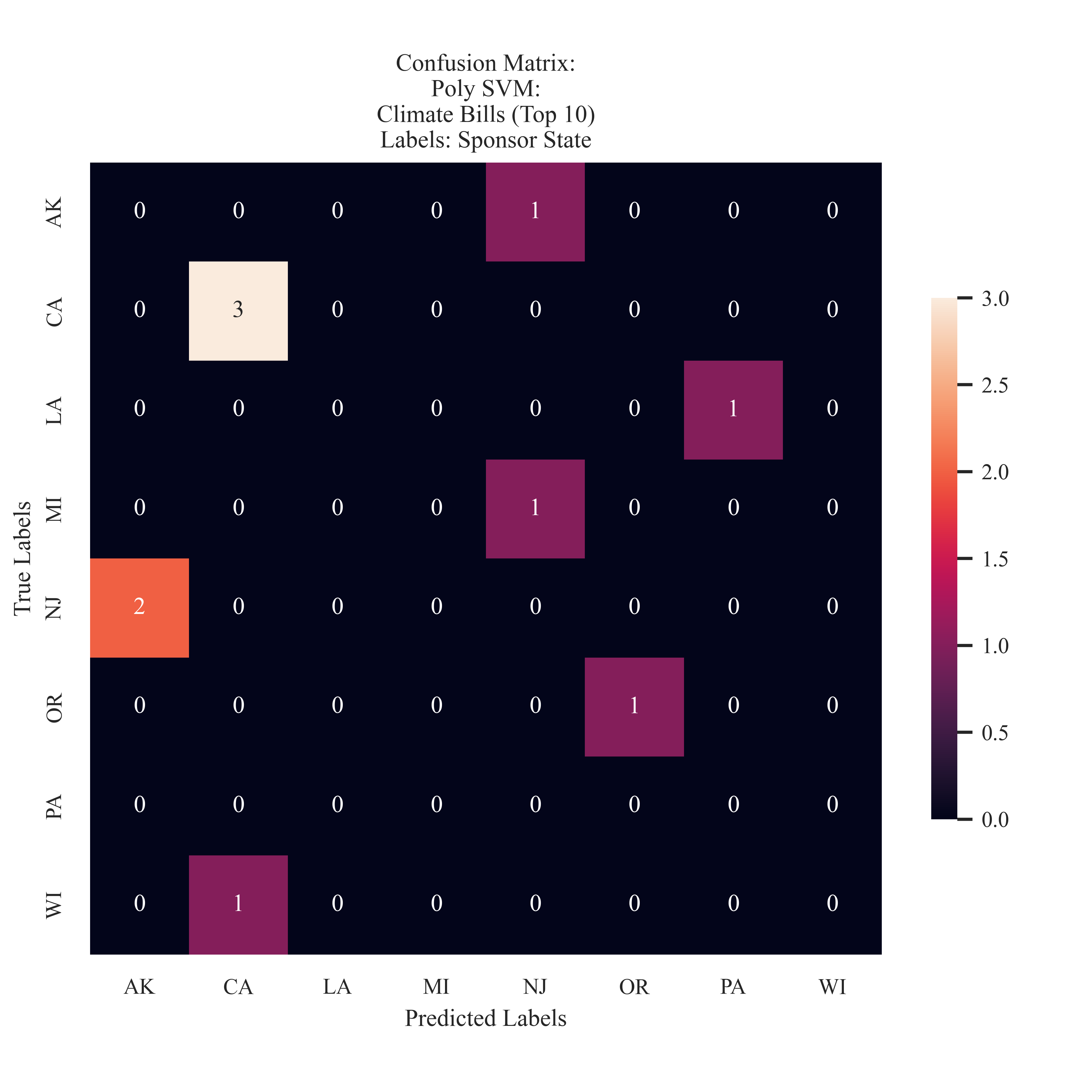
Climate Bills: Sponsor State
The model was unable to learn anything meaningful about State Affiliation, as the confusion matrix is 'randomly' colored.
Conclusions
The questions posed at the start of this introduction focus on how proposed climate bills differ from each other. In what ways may SVM and other supervised learning metrics illustrate polarization and ideological differnces throguh the lagauge used? Using a Polynomial Kernel with cost of 1000 to train an SVM model, an accuracy of 80% was observed for the bill’s sponsor affiliation, 79% for classification of the bill type, and 93% accuracy for sentiment. This model preformed strongly in identifying differences between the imbued labels. These findings suggest that the semantic differences in ideology, or what makes these labels different from each other, are present in the text. The misclassification rates from the sponsor affiliation illustrated the same pattern as observed in the Naive Bayes model. The majority of the misclassificatinos were predicting a Democrat label when it was actually Republican. This could indicate that for some introduced Republican Bills, the difference in language is not as discernable between ideologies. In addition, future research should consider including more Independent labels to better understand the features which compose this parties climate policy ideology.
In comparison to the Naive Bayes model, the SVM model struggled to detect the Sponsor state. While California, had the most classifications, it was only granted a gueses. In addition, the confusion matrix does not demonstrate a clear pattern of learning. It may be suggested that the bill sponsor’s state does not play a strong role in determination, however the preformance of Naive Bayes on the same label suggests otherwise.
The next question considered how features of the news cycle, like named political entity or publisher, impact the semantic paritions that may be identified through the text. The SVM model most accurately predicted Democrat labels. However, it tended to predict the Democrat label more than the total of Republican predictions. This suggests that SVM did not obtain as strong of an understanding about paritisan affiliation in a more ambiguous sample type.
The model preformed the best on Sentiment data. This is a strongsuit of its preformance due to the imbalance that was observed in the sentiment distribution. The model preformed strongly when handling the valence associated with climate bills, and only mislclassifying only 6% of the testing instances. It should also be noted that these were not necessarily ‘lucky guesses’ as the model shared the 93% accuracy into precision and recall metrics. The model did not preform as strong with the news data. It misclassified 10% of the testing instances (more so with predicting a negative label when it was actually positive) and had a range of precision, recall, and accuracy between 53 and 54%.
In sum, the SVM model was able with great accuracy able to predict binary labels, but struggled when predicting labels with multiple options. This may be in part due to the polynomial kernel utilized when looking for patterns in the data.