Political Stances: Naive Bayes
Overview
Naïve Bayes is a machine learning model which uses probabilistic classification to assign a label to a text. Using probability the multinomial model may consider the number of tokens and the probability of the token falling into its respective label. Its naïvety in part due to the few parameters needed to train but also the assumption that the model may then not capture as much nuance within the data as a result of this. (Grimmer et al: 20222). For this project, its simplicity is a strongsuit the linear classifications which are not prone to overfitting.
The questions posed in the introduction are a well suited task for this method. First, considering how climate change is represented requires an understanding of the way in which the text composes the document. Being able to classify the documents into the labels, which were already embedded into the creation of the document, may inform how climate change is represented at the federal level. Next, when considering news polarization with respect to climate change, a strength in classifier performance specifically when delineating descriptions about Republican or Democrat headlines, may support the idea of increased news polarization.
Table of Contents
- Data Preparation
- Method
- Model Evaluation
- A Naive Reading of the News
- Interpreting Features about Climate Bills Naively
- Conclusions
Data Preparation
All supervised learning models (ie, they take label data) require a few things. The first, is a train test parition. This is important because to test the models efficacy it requires an unseen dataset - it not the model is trained incorrectly and is often times overfit. Next, the supervised model requires labels. The data utilized in this project is a combination of News Headlines and Proposed Bills tagged as climate at the federal level. The data may be found either at the in-text links just provided, or at the HuggingFace Collection developed for this project. The prior labels generated for news data are the mentioned partisian affiliation, and the publisher of the news source. For the proposed bills the labels included are the bill sponsor’s state, partisian affiliation, bill type, and hearing committee.
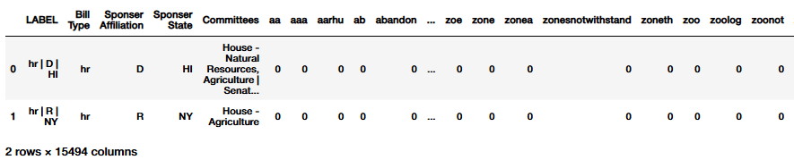
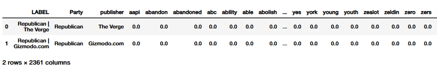
For the purposes of the following machine learning methods, a ‘combined’ metadata label was generated. For all combined labels the token ‘|’ was utilized to split the different labels. This token was selected because of its rarity in the other labels, and a clean way to later visualize the combined labels. An example of news metadata label may be ‘Republican | The Verge’, and for the proposed cliamte bills ‘hr | D | hi’. The combined label for the bills data first represents the bill type, or what chamber it originated from, then the bill sponsor’s partisian affiliation and state. This code is consistent across the entire dataset. The two figures below illustrate the headed versions of the data frames, with their labels preserved. It should be noted that the labels were removed for the classification by the model, or else it wouldn’t work!
To generate a Train Test Split consistently across all of the superivsed models (Naive Bayes, Decision Trees, and Support Vector Machines), a custom function was developed. This function would take a Pandas DataFrame and then the label column. This is used to generate both lists of labels and to then visualizae the distribution of the particular label with respect to the train test split.
The function uses sklearn’s train_test_split with a parition of 30% reserved for testing. The size of the dataset allows for this large of a parition to be taken. The custom function then generates a list of the training labels, and the testing labels. The option to remove the label column is preserved in the function but seldomly used. Finally, the function returns the training data, testing data, and their respective labels stored in separate lists.
def train_test_splitter(data, label_column):

    data_train, data_test = train_test_split(data, test_size = 0.3,)
    labels_train = data_train[label_column]
    labels_test = data_test[label_column]

    #data_train.drop(columns='LABEL', inplace=True)
    #data_test.drop(columns='LABEL', inplace=True)


    return (data_train, data_test, labels_train, labels_test)
Each label had a custom testing and training split, as the model can only handle one label at once (but this was in an attempt to be mitigated by generating the combined ‘metadata’ labels. It is illustrated in the Train and Testing Data Parition Table that regardless of the label, the split generated is the same size every time. In total eight dataframes were generated for each type of label. To then include the testing and training splits, a total of sixteen dataframes were generated.
Train and Testing Data Parition
| Training Data | Testing Data | |
|---|---|---|
| News Headline: Partisian Affiliation | 573 | 246 |
| News Headlines: Publisher | 573 | 246 |
| News Headlines: Publisher and Partisian Affiliation | 573 | 246 |
| Climate Bills: Sponsor Affiliation | 2256 | 967 |
| Climate Bills: Sponsor State | 2256 | 967 |
| Climate Bills: Metadata | 2256 | 967 |
| Climate Bills: Bill Type | 2256 | 967 |
| Climate Bills: Hearing Committee | 2256 | 967 |
The distribution of the Partisian Labels are illustrated below. It is important when developing these models to consider the distribution of the labels within the training and testing sets. If the training sets are disparate this may lead to the model overfitting on a particular label and not ‘learning’ what comprises of the other labels. Provided below are the distributions, specifically for the testing data of the Partisian Labels. For the News Headlines, the distribution is relatively split equally between Republican and Democrat. In comparison to the Proposed Cliamte Bills, the distribution is not as equal - and includes the Indepent Partisian Affiliation. These differences in distribution are not something to necessarily correct - as the goal of machine learning is not to have the model discern half of the data automatically as one label - but to instead be able to learn the semantic characteristics which generate text to be a particular label.
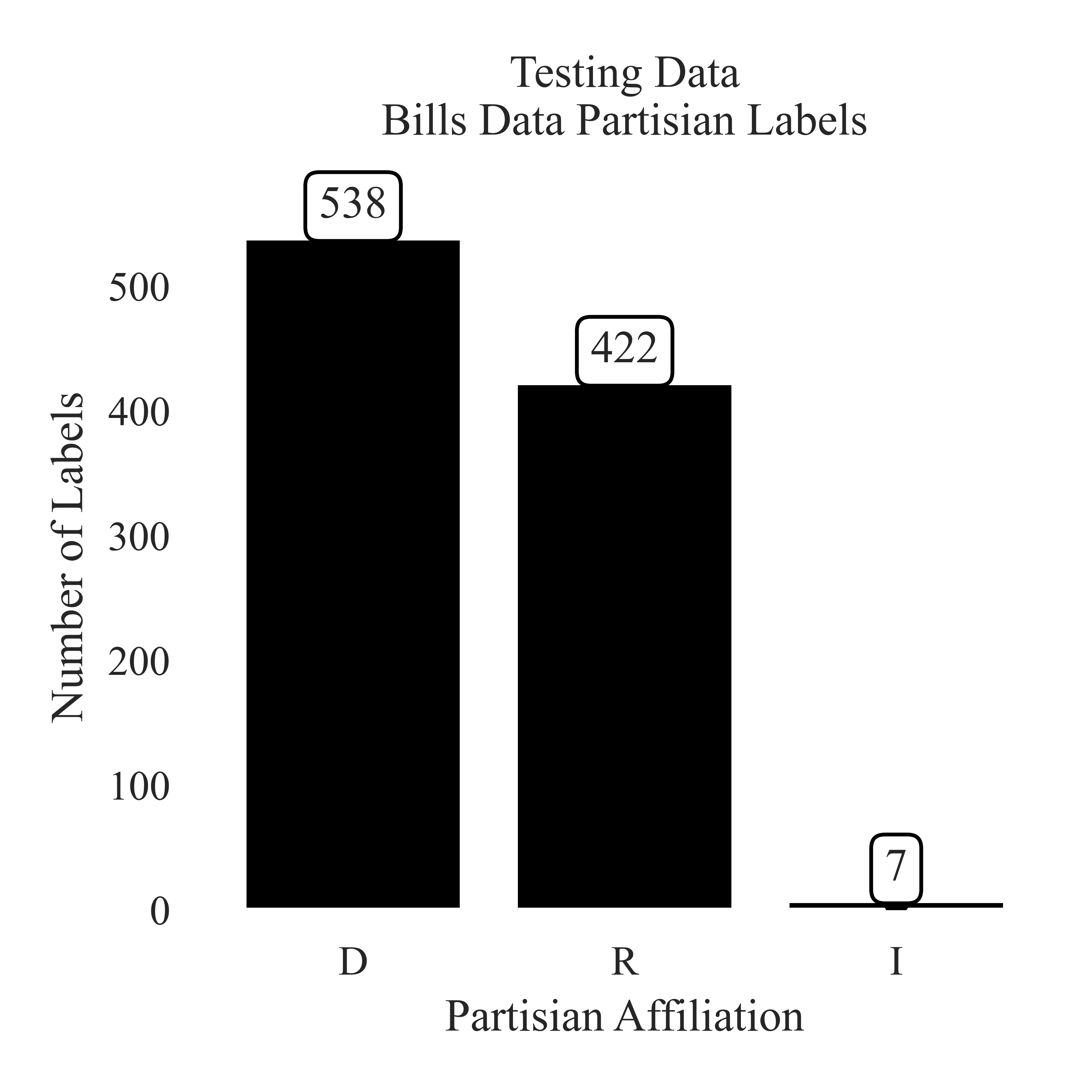
Testing Data Paritisan Label Paritions of Proposed Climate Bills
The Democrat party has 538 testing instances, which is more than the Republican party with 422 testing instances. The Independent party has seven testing instances.
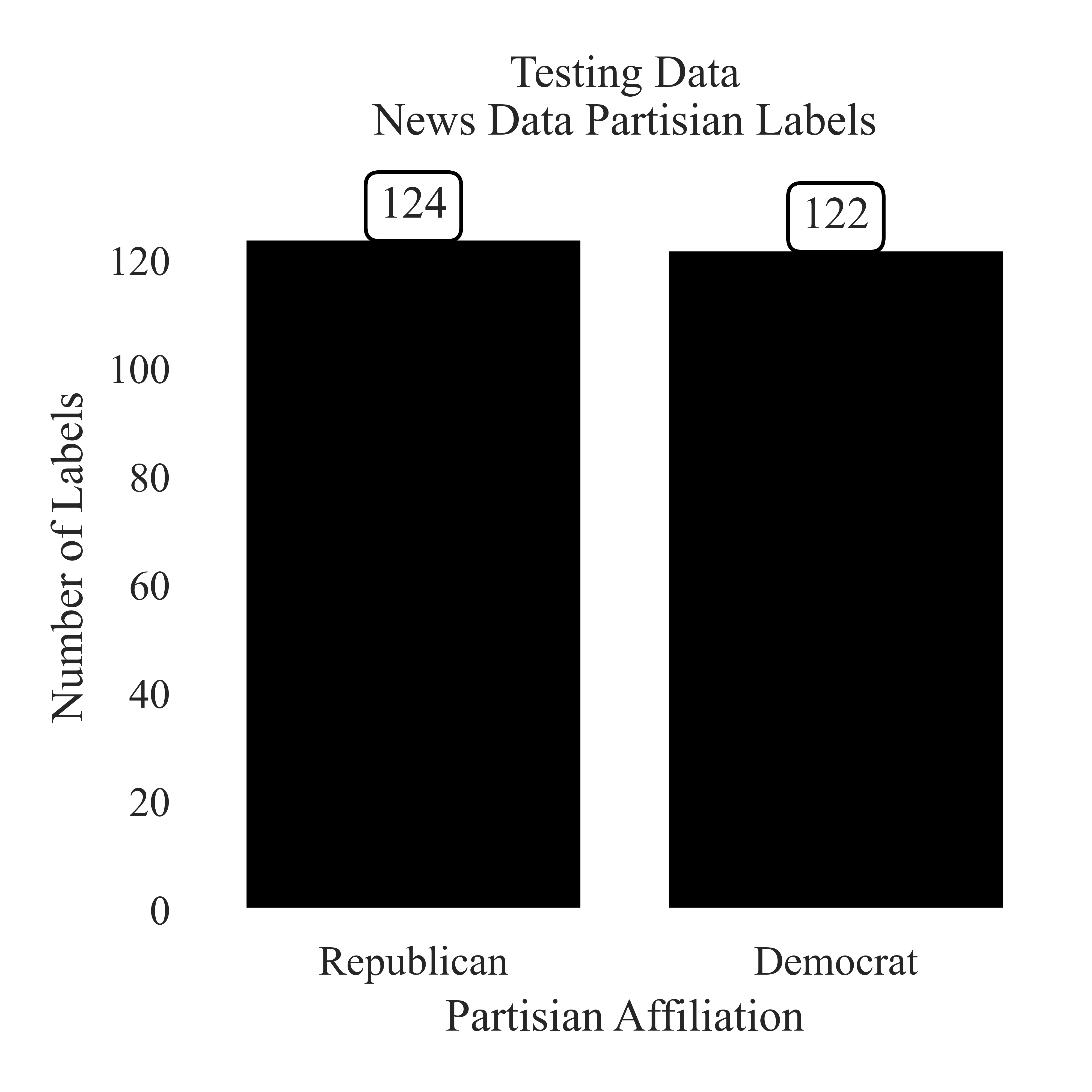
Testing Data Partisian Label Paritions of News Headlines
The distribution of testing data between Republican and Democrat is relatively even. The Republican label has 124 testing instances, and the Democrat label has 122 instances.
Method
The method section is split into two parts, first an explanation of how the MNB models were fit. As noted earlier, there is eight different dataframes which MNB will be trained on, so internal consistency is important - especially when evaluating the performance of different labels tandemly. Next, the evaluation function is described and its application. The Multinomial Naïve Bayes model was selected because of the multiplicity of dimensions and complexity presented in the data.
Systemicatically Fitting the Multinomial Naïve Bayes Models
To systemctically fit the model, a custom function was needed. The idea behind this function was to internally train, assess, and visualize the performance of the MNB with respect to a particular dataset. The first inputs to this function are the training data and testing data, their respective labels. This is essential from training the models and assessing them. Next, the column name is needed for the label, as the function will then drop the labels that were preserved during data preparation. The confusion matrix graph title and file name are the subsequent inputs. The final parameters are used in the generation of the visual confusion matrix, and will be explained in the next section.
After instantiating an unparameratized, or the defaults of MNB provided by SciKit Learn. The model is then trained using the mnb_model.fit() attribute. The predictions are then generated, and passed into the model_verification function and then visualized. The output of the function are the respective precision, accuracy, and recall scores and a confusion matrix both displayed and saved to the local machine.
def mnb_modeler(data_train, labels_train, data_test, labels_test, label_column_name,  graph_title, labels_name, file_name,filter_top_n = False, N=10 ,fig_x = 6, fig_y = 4):
    data_train = data_train.drop(columns = label_column_name).copy()
    data_test = data_test.drop(columns = label_column_name).copy()

    mnb_model = MultinomialNB()

    ## Fitting the data
    mnb_full = mnb_model.fit(data_train, labels_train)

    ## Creating predictions
    predictions = mnb_full.predict(data_test)

    ## Assessing the models abilitiy
    accuracy, precision, recall = model_verification(labels_test, predictions)

    ## Filtering for Clean Visualizations
    if filter_top_n == True:
        labels_test, predictions = filter_top_n_labels(labels_test, predictions, N)

    ## Generating a confusion matrix

    matrix_ = confusion_matrix(labels_test, predictions)
    visual_confusion_matrix(matrix_, labels_test, predictions, graph_title, labels_name, file_name, fig_x, fig_y)

    return (accuracy, precision, recall)
Devoping a System for Model Evaluation
There are three metrics used to commonly assess machine learning models. These are recall, precision, and accuracy. To generate these metrics, the ‘positives’ and ‘negatives’ are calculated. A ‘positive’ may be understood in regards to both a gold (or true) porsitive and a system positive. A ‘negative’ is essentially the other label, or series of them. The overlap between the system and gold positives are referred to as ‘true positives’, however, if the system predicted another label for the label in question, this is referred to as a ‘false negative’. ‘False postivies’ are similar to a ‘false negative’ in the sense that it was an inocrrect prediction for the label. The ‘true negative’ is the pair to the ‘true positive’ and is when the system and gold labels are aligned.
Using a combination of the positive and negative labels, recall, precision, and accuracy may be calculated. Precision is the number of true positives divided by everything the system predicted to be that label. This measures the “percentage of the items that the system detected that are in fact positive” (Jurasky and Martin: 2025). Next, recall is the number of true positives divided by the number of items that had the true positive label. This is measuring “the percentage of items actually present in the input that were correctly identified by the system”. Finally, is accuracy. This calculates how many total correct observations were labeled divided by the size of the corpus. This measures how accuracte the model was with respect to the entire corpus.
The definitions outlined here focus on binary labels (like partisian affiliation), however, when calculating for additional labels marcro averaging is reported - as it demosntrates the general preformance for each class (Jurafsky and Martin: 2025).
Image Source: Jurafsky and Martin, Speech and Language Processing, page 67
To systemtically compute each recall, accuracy, and precision, with a macro average SciKit Learn’s Metrics Package was utilized. for precision and recall, the average was set to macro to ensure correct reporting of the evaluation metrics.
This function was utilized to feed into the visual confusion matrix. Using the predictions, a confusion matrix may be generated to understand how accurate the model is at a glance. The intuition behind these matricies is that the diagonal, going from upper left corner to lower right corner, should have the largest classification of predictions - that is is the model is trained accurately. Any patterns that aren’t necessarily a clean diagonal indicate misunderstandings in the models learning, and deeper discussion should be presented with regards to speculating why the model has learned in the way it did.
from sklearn import metrics
from sklearn.metrics import precision_score, recall_score, accuracy_score,

def model_verification(true_labels, predictions):
    accuracy = accuracy_score(true_labels, predictions)
    precision = precision_score(true_labels, predictions, average='macro', zero_division = 0)
    recall = recall_score(true_labels, predictions, average='macro', zero_division = 0)

    return accuracy, precision, recall
Results
The results section is split into two parts, the first is an evaluation of the Multinomial Naïve Bayes Models’ preformance. Next, a discussion will be presented about the nuance behind the confusion matricies presented. Finally, this page will close with the potential implications of the resutls presented here with respect to the research questions outlined in the introduction.
Assessing the Validity of the Multinomial Naïve Bayes
This results section begins with an assessment of the validity because it is important to hedge the implications of the findings with respect to the preformance of the model. In this section are a figure and a table which will weight the discussion, the information represented in each are the same.
News Headlines The accuracy of the MNB preformance on the model ranged largely. For its ability to classifiy partisian affiliation was about a 58% across all three evaluation metrics. In comparison to the models low (and somewhat abysmal) preformance on the Publisher classification (28% accuracy), and even lower preformance on the metadata classification (17% accuracy), this is the most reliable label for classification. Specualtion may be granted to why the model preformed this way. For the partisian affiliation, often the word ‘Republican’ or ‘Democrat’ may be presented in both news articles. For example, the headline and news snippet: ‘How Biden’s domestic policy record stacks up against public perception,President Joe Biden ends his term with a gulf between his policy record and his public reputation. The Democrat spent so much of his time addressing long…’ (Source: Yahoo Entertainment) is tagged as Republican due to the data collection technique, however the snippet discusses the actions comitted by the Democratic President, Joe Biden. This suggests that while the classifier does have issues , it may be in part due to the labeling scheme originally generated during data collection.
In addition, the low accuracy of Publisher Classification illustrates that there may be some discriminating factors that determine how publications generated content, but it is hard to parse. The slightly higher precision rate demonstrates that the MNB classifier is more likely to predict the true label, than a miscorrect label in the smaller comparison between what the model did get correct. In alignment with the presented logic here, it is expected for the metadata to preform the least successfully. The precision and recall of 0.04% suggests that the model was simply guessing, and happened to get 17% of the training instances correct. If the model was already struggling with the ability to discriminate publisher and partisian affiliation, it would not be expected for the model to preform well on a combination of the two.
Proposed Climate Bills There were five labels tested from the Climate Bill dataset: sponsor affiliation, sponsor state, metadata, bill type, and hearing committee. The classifier preformed the best on Sponsor Affiliation, then second on Bill Type. The accuracy for both of these models was above 70%. The hearing committee had a high accuracy (48%), however, low precision and recall (11%) suggesting that the model had quiet a few lucky guesses. Next was the sponsor state - it had higher precision and recall than the committee label, but a lower accuracy. This may be in part due to the number of label options available to the model (50 states). The nearly eqaul precision and accuracy scores (23% snd 26% respectively) demonstrating the ‘learned’ ability from the model. Similarly to the metadata label from the news headlines, this label preformed the weakest out of the labels (but not as poorly as the News Headlines did). This may be in part due to the observed difficulty of the model predicting the bill sponsor’s state. It may be speculated that if the sponsor state was excluded from the metadata label, the metadata label may have preformed better.
The MNB had more variation of evaluation metrics on Sponsor Affiliation than the news headline did, however, it had a higher accuracy overall. There was 967 instances in the testing data, which means that the model accurately predicted the sponsor’s affiliation correctly 740 times. However, the precision and accuracy sit at 52%, suggesting that the model intentionally predicting just over 500 of the testing samples because of its observed learning. A similar pattern is observed with the Bill Type. The bill type may be understood as where the bill originated from. This label is also representative of if the particular bill is a resolution, which is a different principal form than the bill itself. It has a high accuracy, but lower precision and recall rates at 45% and 46% respectively.
| Accuracy | Precision | Recall | |
|---|---|---|---|
| News Headlines: Partisian Affiliation | 0.577 | 0.578 | 0.577 |
| News Headlines: Publisher | 0.276 | 0.16 | 0.145 |
| News Headlines: Publisher and Partisian Affiliation | 0.167 | 0.035 | 0.038 |
| Climate Bills: Sponsor Affiliation | 0.759 | 0.521 | 0.518 |
| Climate Bills: Sponsor State | 0.255 | 0.23 | 0.171 |
| Climate Bills: Metadata | 0.206 | 0.126 | 0.117 |
| Climate Bills: Bill Type | 0.711 | 0.449 | 0.463 |
| Climate Bills: Hearing Committee | 0.478 | 0.111 | 0.109 |
Considering The Presented Evaluation of the Model The model varied in its preformance. The labels with the highest accuracy was from the climate bills sponsor affiliation, the partisian label from the news headline, and the bill type. It may be expected that in some of the labels, like the metadata for the news headlines, the model did not appropriately learn. This is suspected in the hearing committee classification as well. The following confusion matricies will be used to further illustrate and understand the nuance of these patterns.
A Naive Reading of the News Headlines
Publisher
The most prominent pattern is for the label 'Freerepublic.com'. There is not a clear accuracy diagonal, but there are a few accurate predictions.
Named Political Party
The 'diganoal' of accuracy is illustrate,d however, a majority of the testing samples were misclassified.
Combined Headline Metadata
Similar to the preferencec of 'Freerepublic.com' This is demonstrated in the Combined label too. Nearly all of the predictions are in this column.
If any of the labels are too small to read, feel free to click on the image to expand it! Illustrated here are the confusion matricies generated from testing the News Headlines. For the combined label and the publisher label the classification favored the news source 'Freerepublic.com'. When assessing the pattern identification of the partisianship, it is clear that the majority of the the predictions were correct. There was not a particular trend to overpredicting a particular label - but there were more Democrat predictions than Republican predictions. This is not expected because of balance in the testing set.
The model tended to overpredict for the label ‘Freerepublic.com’. To explore potential causees of this, the testing set was examined. 40 of the samples in the testing dataset did belong to Freerepublic. This may be assumed why there was prediction issues in this case. Outside of the ‘Freerepublic.com’ label, the classifier was able to accurately predict articles from the ‘Americanthinker.com’, ‘Forbes’, ‘Raw Story’ and ‘Yahoo Entertainment’. This suggests that in some cases the model was able to accurately predict the publisher. The model maintained thie preformance for ‘Republican | Forbes’ and ‘Republican | Yahoo Entertainment’. This suggests that the model is able to discern between what partisian affiliation is being discussed and by what news party.
Interpreting Features About Climate Bills Naively
There was five different labels from climate bills: sponsor state, sponsor affiliation, metadata, committee, and bill type. The accuracy for this data was overall higher than the news data, however, it may in part be due to it had ‘more’ chances, because the data had more labels. The highest preforming labels were sponsor affiliaiton, bill type, and sponsor state. It should be noted that in the sponsor state, metadata, and committee were truncated to the top ten labels. These were sorted based on the number of predictions assigned to the testing data, and then sorted from most to least. A custom function was developed to do so, and may be reviewed at the code page.
Bill Sponsor State
A clear diagonal is illustrated from correct classifications. The state which had the most predictions (and most accurate) was Califronia, with 37 accurate classifications. Next was New Jersey with 22 accurate predictions.
Sponsor Affiliation
The facets about an Indepent Bill Sponsor were not learned through training, and no testing predictions were assigned to the party. The most common misclassification for the Independent party was Democrat proposed bills. The Republican party had the most predicted labels, with 166 misclassifications from the democrat party.
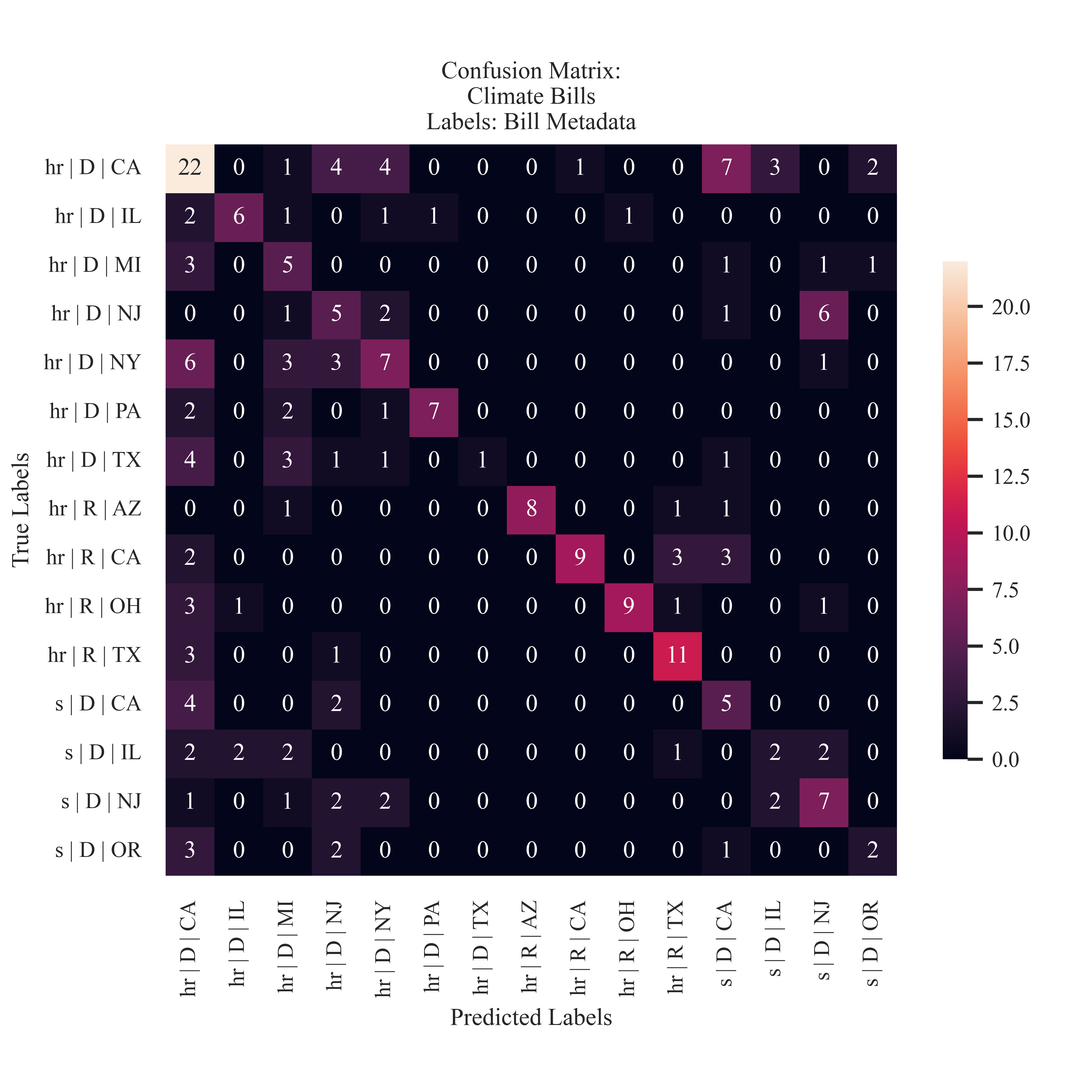
Combined Bill Metadata
A similar pattern is observed from the Sponsor State prediction. Both Democrat and Republican bills were accurately predicted. Something similar is identified with Texas, however the classifier struggled to identify the Democrat sponsored bills. .
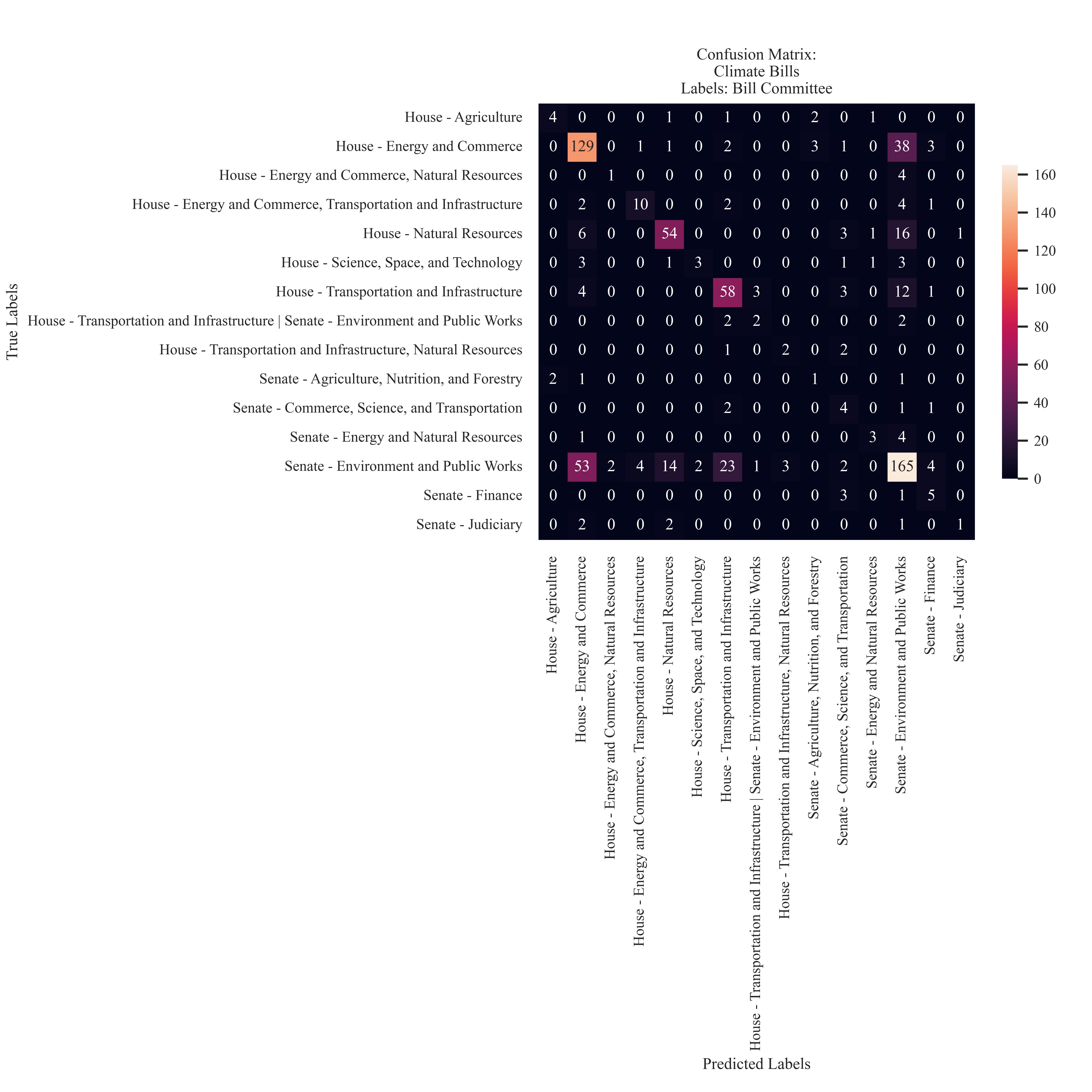
Hearing Committee
The committees with the most predictions were House - Energy and Commerce (129), Senate - Enrvironment and Public Works (165), and House - Transportation and Infrastructure (58). The model had the most success with labels that had a large amount of candidates for classification.
| Abbreviation | Bill Type |
|---|---|
| hconres | Concurrent Resolution Originating From House of Representatives |
| hjres | Joint Resolution Originating from House of Representatives |
| hr | House of Representatives |
| hres | Resolution From House of Representatives |
| s | Senate |
| sconres | Concurrent Resolution Originating From Senate |
| sjres | Joint Resolution Originating from Senate |
| sres | Resolution from Senate |
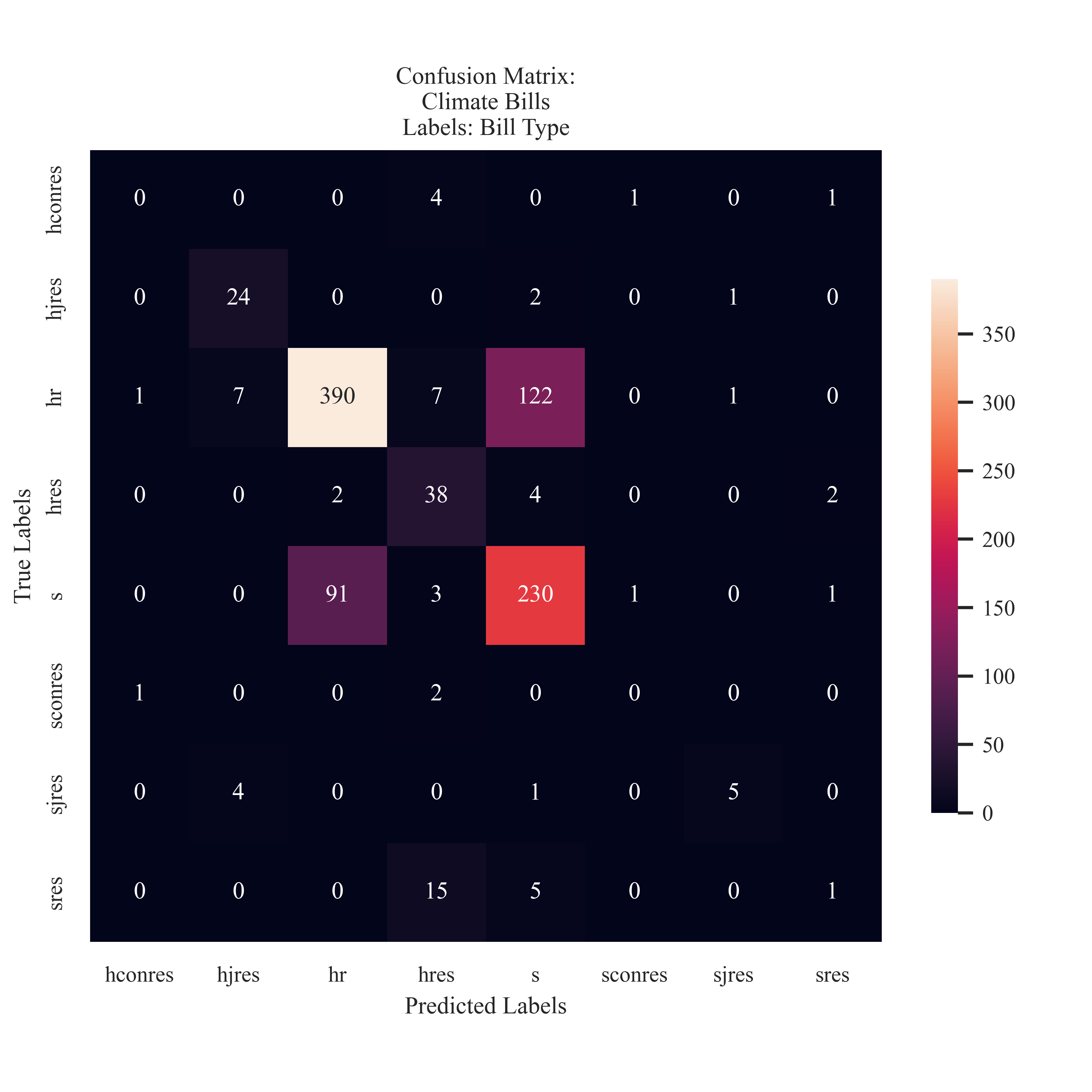
Abbreviation Source: Bills & ResolutionsThe bill type was also considered as a label. The type differs based on where the bill originated from and if it is a resolution.
The classifier had the most success at discriminating between bills introducing from the House of Representatives and the Senate. With some accuracy, it has able to identify jount House Resolutions and House Resolutions. It struggled holistically in identfying differences between Senate introduced bills.
Conclusions
The Naive Bayes model was able to accurately classify partisan labeling present in news headlines and proposed climate bills. The classier was able to most accurately classify news headlines, however had a higher accuracy evaluation rate for proposed climate bills. This finding suggests that the language used to delineate between the two partisian affiliations is clear - polarization was able to be detected in the text. It should be noted that I use polarization here to illustrate difference, not necessarily anomisty. The model struggled to accurately identify the Independent party, however the bills that were introduced by Independnet Sponsors were most often actually Democrat.
This partisian conclusions may be drawn because the model was not able to delineate as well other labels in the text such as the publisher of the news headline or the state which the bill sponsor represents. However, both the bill sponsor state, and the metadata (bill type, partisian affiliation, and sponsor state) both illustrated clear demarcations as the brightest part of the confusion matrix was along the diagonal.
Proposed climate change bills are able to be classified into their respective sponsor characteristics, and in some cases even bill committee. This demonstrates that there is a difference in problematizations which underlie the language used to construct action regarding climate policy. In addition the observed media polarization holds consistent in the findings illustrated here.
Bibliography
Grimmer, J., Roberts, M. E., & Stewart, B. M. (2022). Text as data: A new framework for machine learning and the social sciences. Princeton University Press.
Jurafsky, D., & Martin, J. (2025). Speech and Language Processing (3rd ed.). https://web.stanford.edu/~jurafsky/slp3/ed3book_Jan25.pdf