Political Stances: Decision Trees
Overview
A decision tree is used to identify which features are important in a label. The salient features are those which are discriminating factors to determine what is important to a particular label. For example, a decision tree can provide important information about what is important for ‘Republican’, or a particular news media company.
The discrimate word, or the root node, is used as the original split for the classification path. The features included in a decision tree subsqeuntly then show ‘lef nodes’ which are further paritions of the root node. The tree will then generate until the paritions are no longer fit (either decided through parameters or the data is exahusted).
The nodes generate a parallel leaf which illustrate the change of a particular item, with respect to the other options that are available to it. For this example the chance is demonstarted in the node on the right. Until the leaf reaches its final node, the chance is not yet illustrated clearly through a special model type, samples, and class nodes.
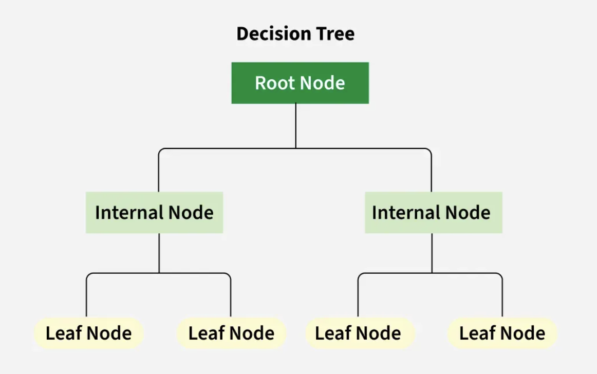
Decision Tree Structure
Image Citation: Geeks for Geeks Decision Tree
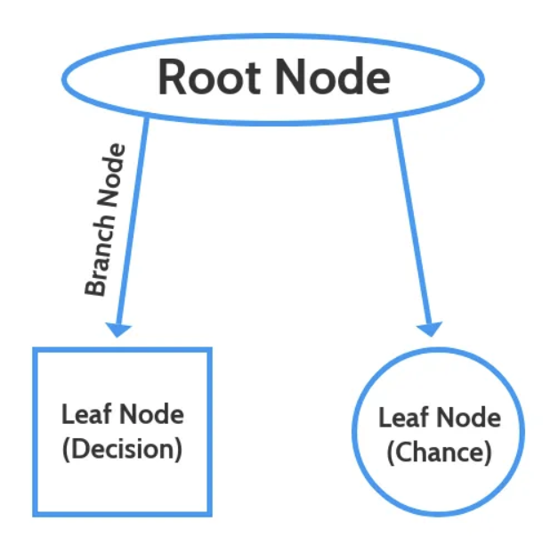
Decision Tree Nodes
Image Citation: Abhigyan "Understanding Decision Tree!!"
Table of Contents
- Data Preparation
- Method
- Evaluating The Gini and Entropy Decision Trees
- Decision Tree Confusion Matricies
- Branching of Labels: Visualizing Salient Factors
- Conclusions
Data Preparation
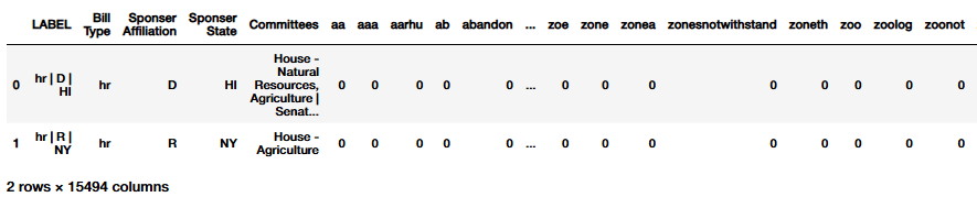
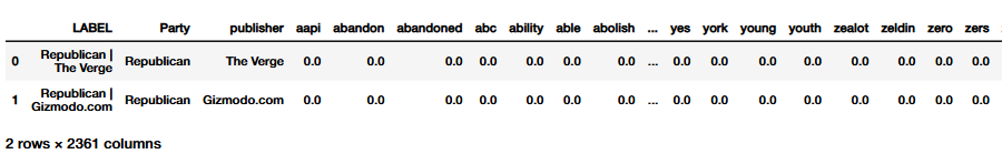
Data was prepared using the same functions outlined in great detail in the Naive Bayes model. It can be reviewed here, or in any of the linked notebooks. The training and testing split is similar to that of the Naive Bayes model as well. A headed version of the dataframes are provided here alongside with the distribution of the train, test, split.
Train Test Split Distribution
| Training Data | Testing Data | |
|---|---|---|
| News Headline: Partisian Affiliation | 573 | 246 |
| News Headlines: Publisher | 573 | 246 |
| News Headlines: Publisher and Partisian Affiliation | 573 | 246 |
| Climate Bills: Sponsor Affiliation | 2256 | 967 |
| Climate Bills: Sponsor State | 2256 | 967 |
| Climate Bills: Metadata | 2256 | 967 |
| Climate Bills: Bill Type | 2256 | 967 |
| Climate Bills: Hearing Committee | 2256 | 967 |
The same naming scheme and train and test scheme were applied across all machine learning methods applied here. This is in order to be able to compare the methods and discuss the original nuance between them. For all three methods, the exact same data preparation was applied - which is why it is not repeated here.
Method
A Decision Tree Modeler was developed similar to that of the systematic testing developed in Naive Bayes Modeling. The Decision Tree used to classify the data was from SciKit Learn’s DecisionTreeClassifier. Both the Entropy and Gini models were tested. The splitter was set to ‘best’ , in opposition to the ‘random’ node split. The max depth was then limited to 7 for Decision Tree readability. The minimum samples split and leaf were inflated to ten. This is because of the scope and number of features in the dataset. The data was also limited to 500 maximum features in order to extract the most frequent commonalities between the data. The max leaf nodes and the minimum impurity decrease were set at the defaults from SciKit Learn. Finally, the class weight was balanced in order to normalize the differences in label distribution. In order to preserve systematic testing, a random state was set to thirty. The random state was able to preserve the essence of ‘randomness’ across the nuancce within the data.
## Decision Tree Modeler:
def tree_modeler(data_train, labels_train, data_test, labels_test, label_column_name, graph_title, labels_name, file_name,filter_top_n = False, N=10 ,fig_x = 6, fig_y = 4):
data_train = data_train.drop(columns = label_column_name).copy()
data_test = data_test.drop(columns = label_column_name).copy()
feature_names_train = list(data_train.columns)
feature_names_test = list(data_test.columns)
decision_tree = DecisionTreeClassifier(criterion='entropy', ## This is changed based on the model test that was used
splitter = 'best',
max_depth = 7,
min_samples_split = 10,
min_samples_leaf = 10,
max_features = 500,
random_state = 30,
max_leaf_nodes = None,
min_impurity_decrease = 0.0,
class_weight = 'balanced')
## Fitting the data
decision_tree_model = decision_tree.fit(data_train, labels_train)
tree.plot_tree(decision_tree,feature_names = feature_names_train)
plt.savefig(f"Decision Tree - {file_name}.png")
## Plotting the tree
dot_data = tree.export_graphviz(decision_tree_model, out_file=None,
feature_names=feature_names_train,
class_names = [str(cls) for cls in decision_tree_model.classes_],
filled=True,
rounded=True,
special_characters=True,
label='all', proportion = True
)
cleaned_dot_data = re.sub(r'value = \[[^\]]*\]<br/>|value = \[[^\]]*\]<br/?>', '', dot_data)
graph = graphviz.Source(cleaned_dot_data)
graph.render(f"Decision Tree - {graph_title}",cleanup=True)
## Creating predictions
predictions = decision_tree_model.predict(data_test)
## Assessing the models abilitiy
accuracy, precision, recall = model_verification(labels_test, predictions)
## Filtering for Clean Visualizations
## Filtering for Clean Visualizations
if filter_top_n:
# Call filter_top_n_labels to get filtered labels and predictions
labels_test_filtered, predictions_filtered = filter_top_n_labels(labels_test, predictions, N)
# If data remains after filtering, create the filtered confusion matrix
if len(labels_test_filtered) > 0 and len(predictions_filtered) > 0:
visual_confusion_matrix(labels_test_filtered, predictions_filtered,
f"{graph_title} (Top {N})", labels_name,
f"filtered_{file_name}", fig_x, fig_y)
else:
print(f"[Warning] No data left after filtering top {N} labels — skipping confusion matrix.")
else:
# If no filtering is needed, generate confusion matrix with all data
visual_confusion_matrix(labels_test, predictions, graph_title, labels_name, file_name, fig_x, fig_y)
return (accuracy, precision, recall)
Evaluating Gini and Entropy Decision Trees
The precision, recall, and accuracy measures will be reported and compared. By an initial look at the bar charts, it is evident that the model only learned features about paritisan affiliation in news, bill sponsor affiliation and bill type. The preformance of all of the other models illustrate a failure of learning for the more complicated labels such as sponsor state or bill hearing committee.
In this section,first, the evaluation metrics will be reported for the entire set, and then for the three models which had non-zero (some learning) preformance.
| Gini | Entropy | |||||
|---|---|---|---|---|---|---|
| Accuracy | Precision | Recall | Accuracy | Precision | Recall | |
| News Headlines: Partisian Affiliation | 0.585 | 0.621 | 0.607 | 0.585 | 0.621 | 0.607 |
| News Headlines: Publisher | 0.008 | 0 | 0.011 | 0.004 | 0.002 | 0.01 |
| News Headlines: Publisher and Partisian Affiliation | 0.008 | 0 | 0.008 | 0.004 | 0 | 0.008 |
| Climate Bills: Sponsor Affiliation | 0.454 | 0.44 | 0.478 | 0.434 | 0.396 | 0.457 |
| Climate Bills: Sponsor State | 0.033 | 0.019 | 0.019 | 0.034 | 0.035 | 0.049 |
| Climate Bills: Metadata | 0.029 | 0 | 0.005 | 0.017 | 0.009 | 0.036 |
| Climate Bills: Bill Type | 0.09 | 0.353 | 0.305 | 0.461 | 0.309 | 0.293 |
| Climate Bills: Hearing Committee | 0.022 | 0.002 | 0.014 | 0.009 | 0.012 | 0.047 |
Gini Model Evaluation
Average Full Model Preformance
- Accuracy: 10.18%
- Recall: 18.12%
- Precision: 17.8%
Average Learned Label Preformance
- Accuracy: 37.33%
- Recall: 46.33%
- Precision: 47%
The overall preformance of the model is poor. The evaluation metrics, specicially that of precision and recall, demonstrate that the model did not learn in many facets. It preformed the best on partisan affiliation for both cliamte bills and news headlines. The Gini model preformed the same on News Headlines paritisan affiliation as Naive Bayes (58%) but had a lower accuracy on climate bills (compared to 76%). The Gini Model preformed stronger than the SVM model on News Headlines (54%) but lower on Bill Sponsor evaluation (compared to 80%).
This demonstrates that in comparison to the other models utilized, and for this data, that the Gini Model would not be appropriate to draw accurate conclusions on.
Entropy Model Evaluation
Average Full Model Preformance
- Accuracy: 19.12%
- Recall: 18.5%
- Precision: 17.37%
Average Learned Label Preformance
- Accuracy: 49%
- Recall: 45.33%
- Precision: 44.33%
The Entropy model had stronger preformance than the Gini model. It specically increased the ability to classify the Bill Type imprving the Gini accuracy from 9% to 46%. However, ‘better’ does not necessarily mean the model would be able to reliably classify, as while the accuracy is higher the precision and recall averages are both lower. In comparison to the aforementioned comparison between Naive Bayes and the SVM models, the Entropy Model mirrors the preformance of the Gini. The difference lies in the ability for Bill Type Prediction. The Entropy model preforms at an evaluation of 31% (P), 46% (A), and 29% (R). When comparing to the Gini, the models have similar accuracy and recall (35% and 30% respectively), but do not preform as well as the Naive Bayes Model (45% P, 71% A, 46% R) or the SVM Model (76% P, 79% A, 69% R).
The classifications observed by the evaluation metrics for both Gini and Entropy illustrate that the data may not be a good fit for the Decision Tree model.
Label Classification: Consufion Matrix Comparison
Presented above are the limitations of the Decision Tree method through the framework of evaluation metrics. Presented below are the confusion matricies which will contextualize these errors. The discussion presented here is caveated with an understanding of the above (atrocious) preformance metrics.
Gini Partisian Affiliation Labeling for Climate Bills
The model was more likely to predict the Democrat Label than the Republican Label. Many of hte misclassifications were of the Independent party. Many of the true Democrat labels were predicted as Republican - more so than the predictions of the the true Democrat label. This suggests that the model favored the Republican party when assigning classificatons.
Entropy Partisian Affiliation Labeling for Climate Bills
The Entropy model follows a similar trend as the Gini model. The Entropy model was not able to accurately predict the Republican model as well, and has more Democrat and Independent mis-predictions than the Gini Model. The preformance of the Democrat label increased, with less misclassifications than the entropy model.
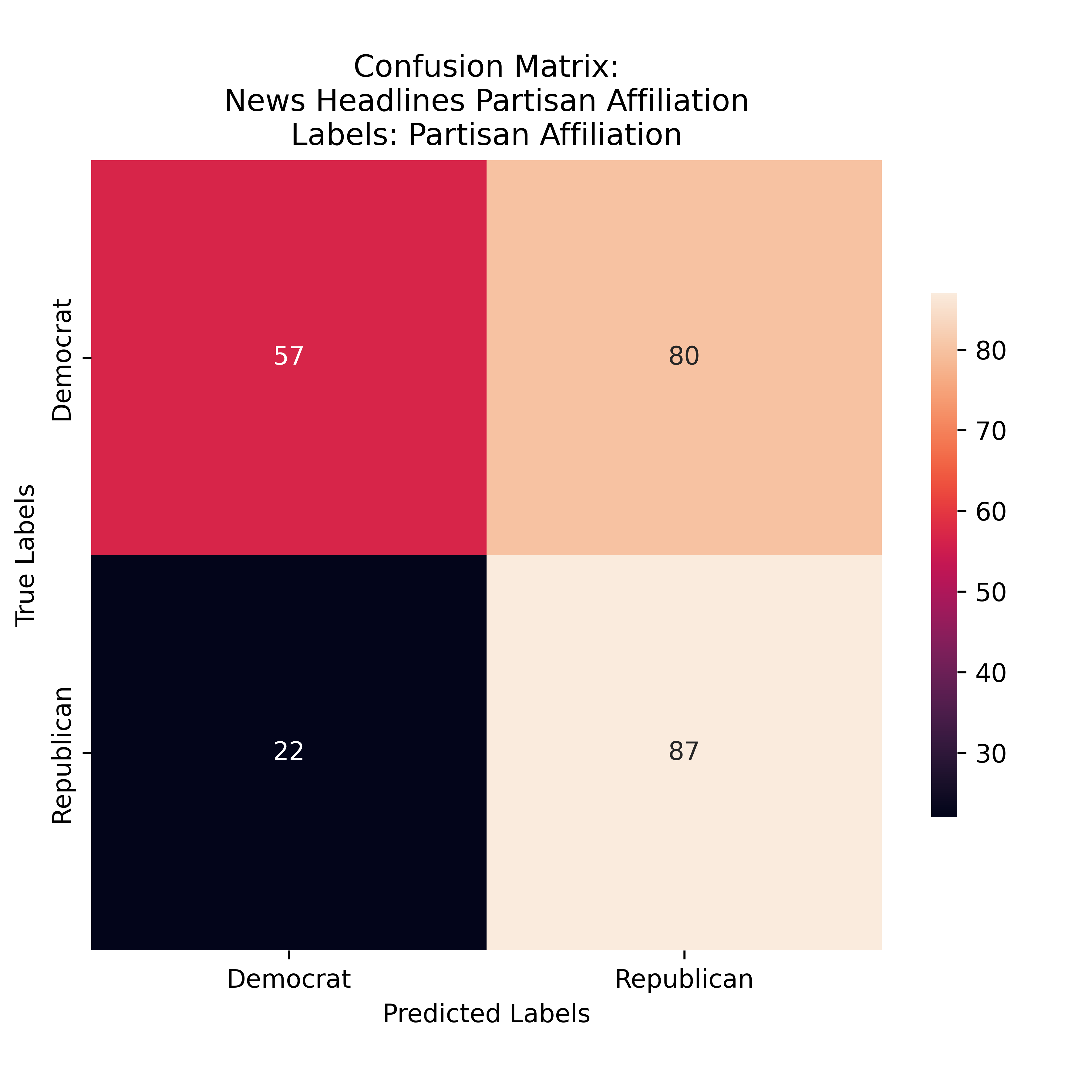
Gini Partisian Affiliation Labeling for News Headlines
The Gini model again favored Repblican Predictions, but matched the preformance of the Entropy Model exactly. This is interseting and suggests that there are som esaleint features which were confusing the models when deliniating between media origented predictions.
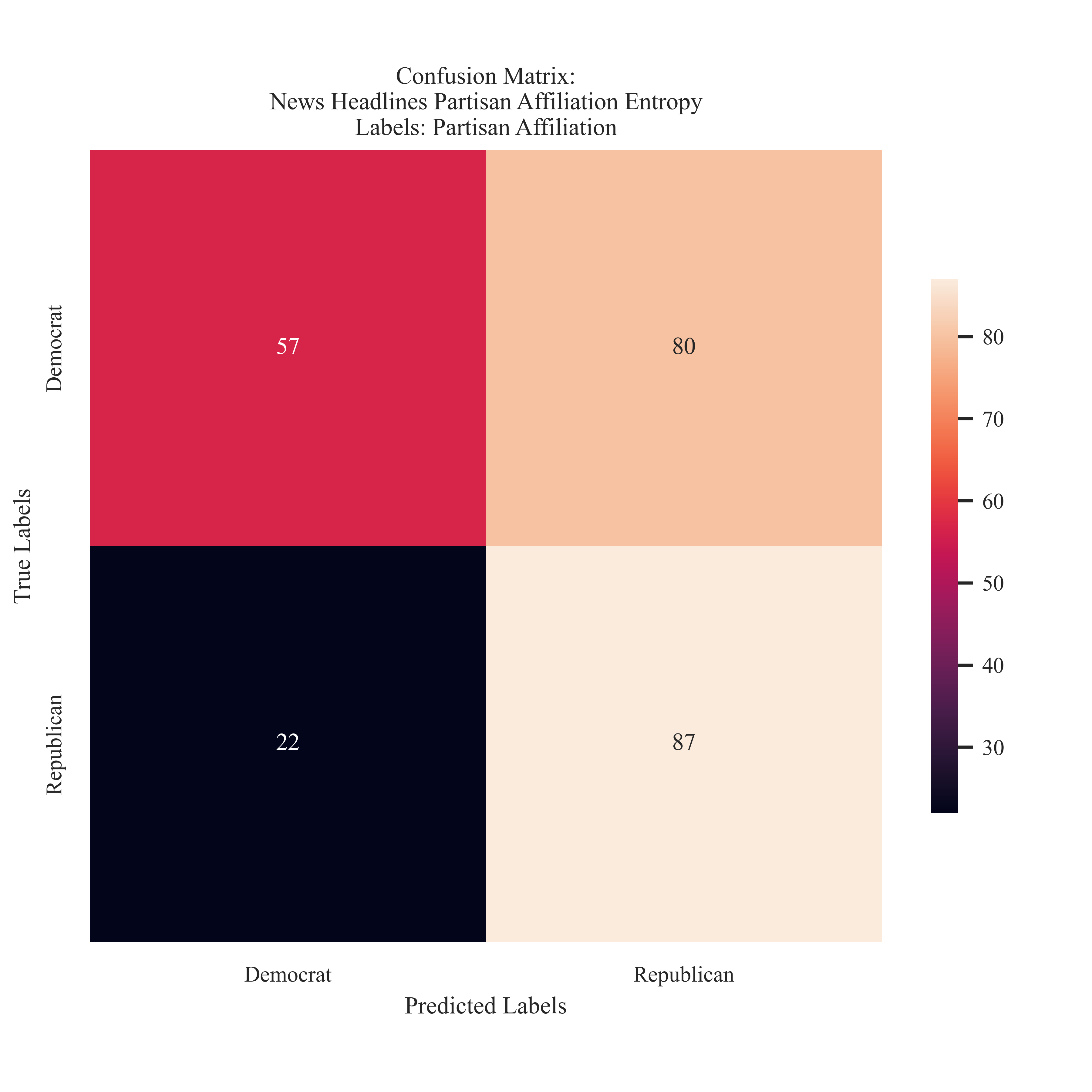
Entropy Partisian Affiliation Labeling for News Headlines
Both the Gini and Entropy models struggled to accurately predict the Democrat Label and had the most false negatives in that category.
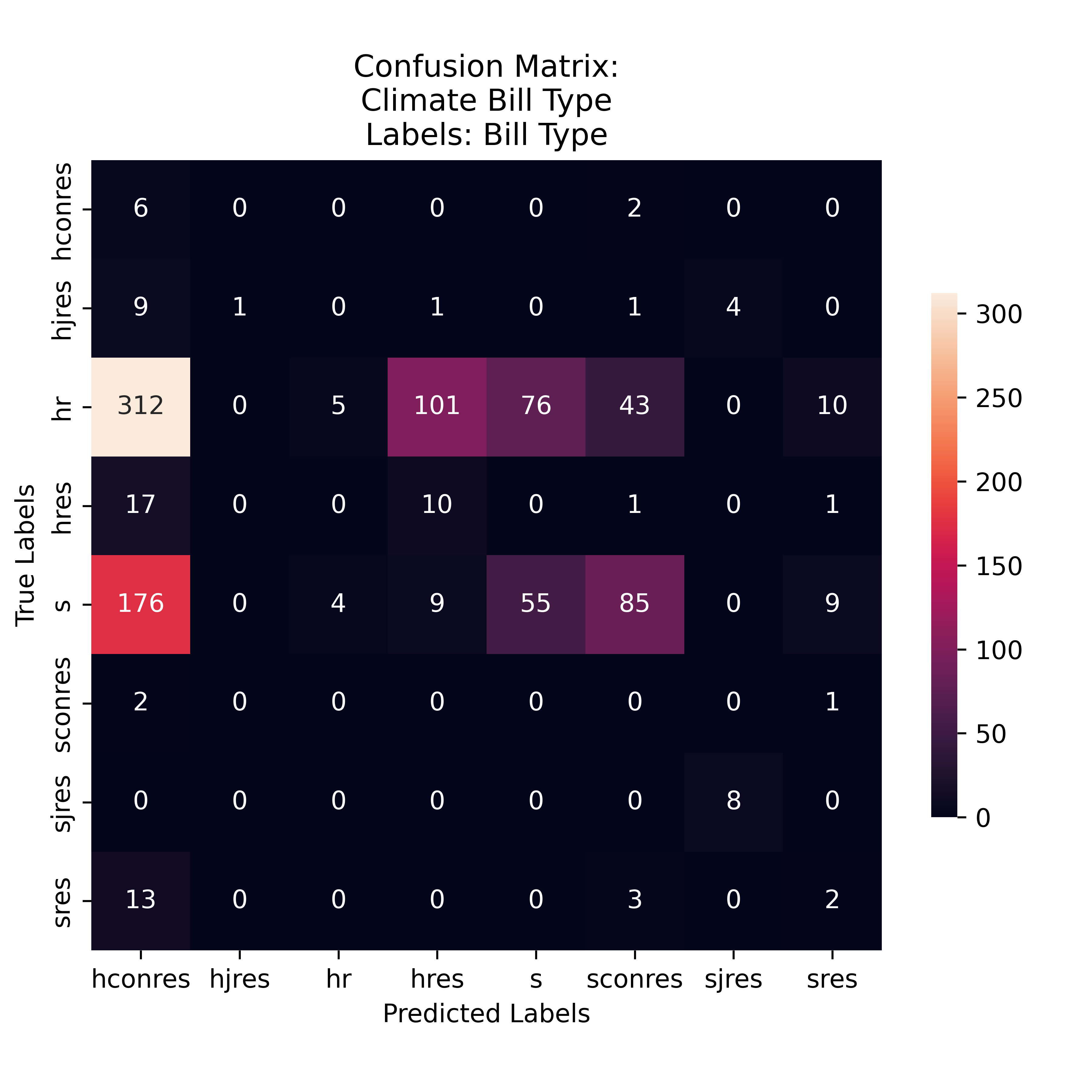
Gini Proposed Bill Type Labeling
The Gini Model was most sensitive to HR predictions, however, many of which were misclassifications for the HConRes. The model was most likely to predict the labels 'HConRes', 'S', and 'SConRes'. Illustrated from the preformance metrics, many of these were just by chance guesses as the precision and recall are rather low.
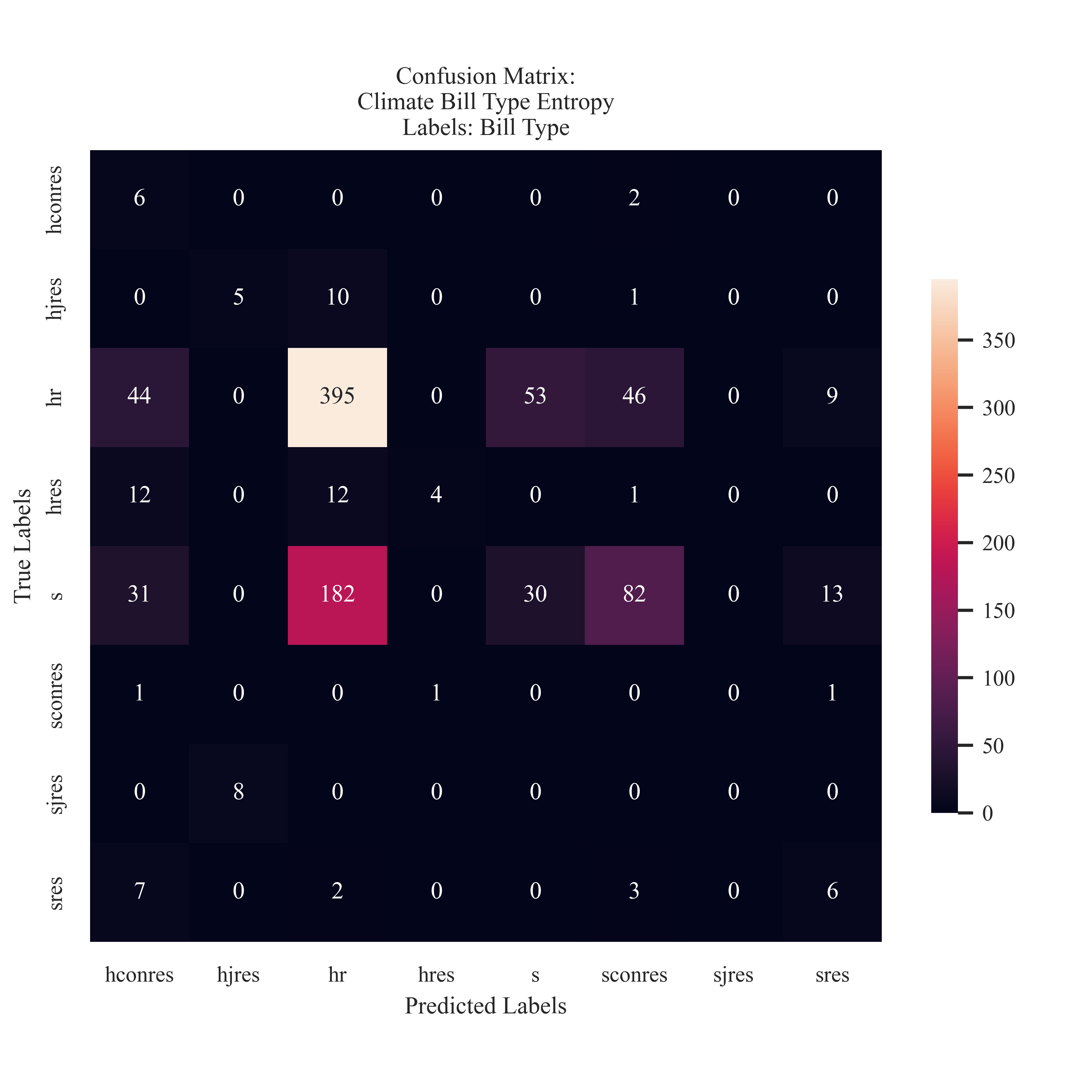
Entropy Proposed Bill Type Labeling
The Entropy Model favored the HR label. It was ale to accurately predict 73% of the bills that originated from the House of Representatives. The mdoel frequently confused the HR proposed bills with S proposed. This is different than the Gini model due to the attention to the larger points of origination in comparison to the resolutions.
View Table Explaining Bill Types
Decision Tree Visualization
Due to the lower results of the ability to classify across many labels, the decision trees illustrated here are the only models that may be assumed were not direct guesses, and illustrative of the models ability to learn. To generate these visualizations, the values (or impurity) scores were removed, and the class name was added to the node in order to identify more clearly the detail within the tree. If any of the words are truncated, it is because the original data was lemmatized. This encapsulates multiple wordforms and helps to demonstrate the root idea. For example, the lemma ‘extrem’ may represent any of the words ‘extreme’, ‘extremely’, or ‘extremital’. These variations are used in many other NLP studies, which is why they are left in lemma form here.
The measure ‘entropy’ will be discussed to contextualize the trees. Entropy is the calculation of how random or uncertain something is. This is then calculated using a randomly selected probability for the selected instance to belong in the class. With respect to decision trees, entropy may be understood as information gain, and representative of how important the feature is. This is in part random, as we have constructed language, however, its randomness provides important semantic meaning to the narrative of the particular text. As best described:
“The entropy has its maximum value when all probabilities are equal (we assume the number of possible states is finite), and the resulting value for entropy is the logarithm of the number of states, with a possible scale factor like kB.”
(MIT Information Entropy Course Notes, CH 10)
This essentially means that the maximum value of entropy is dependent on the number of classes, or labels, which are present in the dataset.
Note: If the browser you are working in does not display the PDFs, they work in Chrome, thank you
Decision Tree: Bill Sponsor Affiliation
The Bill Sponsor Information Root Node beings with ‘temperatur’ starts with an entropy of 1.585. This is less than the entropy in the folllowing root node for Bill Type. The next leaf node is split between the Republican Label or the Independent Label. The node is the ‘disabl’. This than roots into the Republican or Independent Class. It Is not until a depth of three until the Democrat label is mentioned. Once it is, the words which are illustrative of the Democrat label are ‘literaci’, ‘barrag’, ‘taken’, ‘past’, and ‘extrem’. words which are important to the Republican label are ‘program’, ‘capito’, ‘fall’, ‘deriv’, ‘network’, and ‘box’.
The words identified as salient here are different than that in the LDA clustering and Association Rule Mining.
Decision Tree: Bill Type
The root node for bill type is “SJRES”, or Senate Led Join resolution, which then leafs into the ‘HCONRES’ or “HJRES”. It is determined that the lemma ‘hollen’ is salient in identifying this distinction, however the lemma is 2.916. When exploring the tree, some of the words are more representative of that of those in the LDA clustering, like ‘famil’ (HR), ‘construct’ (SCONRES), or ‘damag’ (HR).
In comparison to the tree generated for both Sponsor Affiliation and News Headlines, the tree is more diverse and illustrative of the multi-class complexity when discriminating between proposed bill types.
Decision Tree: News Headlines
The root node for news headlines considers the word ‘angeles’ (D). The leaf nodes split and interesting illustrate the next word as ‘democrat’ with an entropy of 0.999 for the class ‘Republican’. This may illustrate the interconnectedness and complexity of media polarization. The next splits are wildfire (R), Biden (R), right (R), president (D), or watch (R). This data was collected shortly after the Los Angeles wildifres, which may shape the output of the decision tree.
Conclusions
For the collected data, the Decision Tree model preformed poorly. It did not preform competitvely with SVM or Naive Bayes. In addition, in the cases which it had similar accuracy, the other preformance metrics were decreased. It is suggested to consider the illustration of patterns within this dataset less so through the framework presented here.
In response to the physical nodes that were provided in the visualizations, they are logical, however are not aligned with the clustering methods which are presented in earlier stages of this analysis. It would be intresting to consider how these relate to each other in an attempt to holistically answer the research questions presented in the introduction.